P. B. Keegstra, C. L. Bennett,
G. F. Smoot
Hughes STX Corporation
Laboratory for Astronomy and Solar Physics,
NASA/Goddard Space Flight Center
Lawrence Berkeley Laboratory, University of California,
Berkeley
The National Aeronautics and Space Administration/Goddard
Space Flight Center (NASA/GSFC) is responsible for the design,
development, and operation of the Cosmic Background Explorer
( COBE). Scientific guidance is provided by the
COBE Science Working Group.
GSFC is also responsible for the development of the analysis
software and for the production of the mission data sets.
The DMR instrument measures differences in signal between pairs of antennae 60^o apart on the sky. The 53 and 90GHz receivers are sensitive to linear polarization. The microwave signal measured by each antenna of a pair has its E-vector lying radially outward from the spacecraft spin axis.
Because the DMR instrument is differential and every pixel is
multiply sampled, sky maps are produced by solving a coupled
system of linear equations (the normal equations) to minimize
a chi-squared. This procedure can be extended
to account for the additional degrees of freedom represented
by polarization. The signal observed by a radiometer
through an antenna pointed at a particular pixel varies with the orientation
angle  as
as
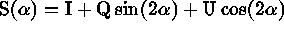 .
I, Q, and U are Stokes parameters representing the state of linear
polarization, and
.
I, Q, and U are Stokes parameters representing the state of linear
polarization, and  is the angle between a vector in the plane of the
radiometers and a fiducial vector on the sky for this pixel.
Since each pixel is observed with a range of values of
is the angle between a vector in the plane of the
radiometers and a fiducial vector on the sky for this pixel.
Since each pixel is observed with a range of values of  ,
recovery of polarization information is possible.
We define our fiducial vector to point from the center of each pixel
towards the north pole. (Our usage differs by a factor of two from
Born & Wolf (1975) so that we can identify the sky map of I with the
DMR sky map made ignoring polarization.)
,
recovery of polarization information is possible.
We define our fiducial vector to point from the center of each pixel
towards the north pole. (Our usage differs by a factor of two from
Born & Wolf (1975) so that we can identify the sky map of I with the
DMR sky map made ignoring polarization.)
From the formula for the signal detected at each pixel, one can construct and minimize a chi-squared to generate the normal equations whose solution gives maps of I, Q, and U on the sky. These normal equations are analogous to the equations for a conventional DMR unpolarized sky map, except that each pixel now has three parameters (I, Q, and U) rather than a single temperature. The correlation of these parameters means that there are nine times as many elements in the normal equations. For example, the single element representing the plus pixel (pixel viewed by the antenna which contributes positively to the difference) by minus pixel off-diagonal contribution to the normal equations for a single observation becomes the following 3 by 3 submatrix:
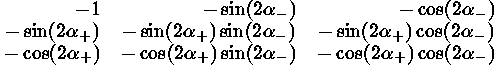
where  is the angle for the plus antenna, and
  the same
for the minus antenna.
the same
for the minus antenna.
The normal equations matrix is the sum, for all observations, of these
contributions. The condition required to obtain a useful solution is that
each time the same pair of pixels are observed, the same values of  must be used in evaluating the contribution to the normal equations. Note
that the orientation
of the spacecraft, and hence the angles
must be used in evaluating the contribution to the normal equations. Note
that the orientation
of the spacecraft, and hence the angles  for the plus and minus
antennae, are fixed by specifying the pointing of the plus and the minus
antennae. Thus one way to satisfy the condition for obtaining a useful
solution is by specifying that the angles
for the plus and minus
antennae, are fixed by specifying the pointing of the plus and the minus
antennae. Thus one way to satisfy the condition for obtaining a useful
solution is by specifying that the angles  be calculated on the
assumption that the antennae are pointing towards the centers of the pixels
they are piercing.
be calculated on the
assumption that the antennae are pointing towards the centers of the pixels
they are piercing.
The effect of this condition on the normal equations is
to make the off-diagonal elements of the final summed
matrix integral multiples of the above 3 by 3 matrix,
where the multiplier is the number of times that the two pixels
were observed together.
Note that all the columns and rows of the above explicit
3 by 3 matrix are multiples of each other. This condition
would not hold in the final summed matrix
if not all  and
and  were equal.
Since the DMR instrument is differential, it must follow that it cannot measure the absolute level of the sky temperature. Phrased another way, the average temperature of the pixels in a conventional DMR unpolarized skymap is not constrained by the DMR data. This is reflected in the algebraic form of the normal equations matrix, so that, if one were to diagonalize the matrix, one would find a single eigenvector whose eigenvalue was identically zero, and the associated eigenvector, viewed as a sky map, would have a constant value.
The added symmetry of the polarization normal equations means that in this case there are six null eigenvectors, the above mentioned map with constant I, and five additional maps with more complicated patterns. These maps are shown in the figures; since eigenvectors are dimensionless patterns, the grayscale value represents arbitrary units.
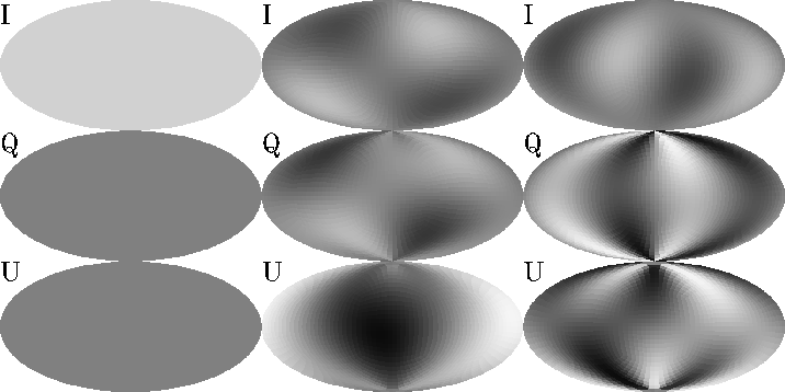
Figure: First, second, and third null eigenvectors.
Each vector consists of projections of the full sky for each
of I, Q, and U.
Original PostScript figure (2386 kB)
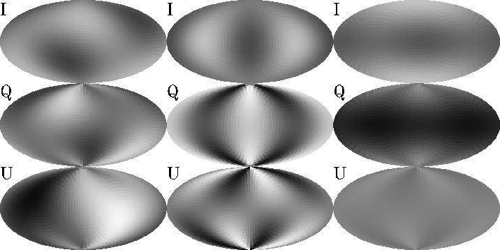
Figure: Fourth, fifth, and sixth null eigenvectors.
Original PostScript figure (2386 kB)
Care must be taken to preserve the symmetry which gives rise to
these null eigenvectors, since this represents a genuine ambiguity
in the experiment. Forcibly breaking the symmetry by using different
values of  for different observations of the same pair
of pixels will not produce any new information, but rather will
cause large amounts of these null eigenvectors to couple into the
final output map.
for different observations of the same pair
of pixels will not produce any new information, but rather will
cause large amounts of these null eigenvectors to couple into the
final output map.
The condition imposed by the iterative solution algorithm is approximately that the projection of the null eigenvectors on the I, Q, and U maps taken together, is zero. This can leave large contributions from the null eigenvectors in the Q and U maps, so long as these are offset in the I map. Since we can calculate the I map much more reliably without polarization, what we are most interested in from these calculations is maps of Q and U. Consequently, as our final step in producing polarized maps, we explicitly project out the contribution of the null eigenvectors over the subspace consisting of just the Q and U maps.
The 53 and 90GHz radiometers of the COBE DMR instrument are sensitive to linear polarization. It is straightforward to define the matrix system whose solution gives best fit solutions for I, Q, and U skymaps. However, the fact that these equations require a 3 by 3 floating-point submatrix rather than a single integer for each off-diagonal pair means that the memory requirements for solving these systems at the standard DMR resolution, using 6144 pixels, are not achievable. Since the memory required scales as the number of pixels to the three-halves power, reducing the size of the calculation one step, to 1536 pixels, allows the calculation to be tractable. To minimize the effect of temperature gradients over these larger pixels, and also to reduce cross-talk into the Q and U maps, the best estimate of the sky temperature from a standard resolution map is subtracted from each data point.
The correct prescription for formulating the model functions associated with each observation has been obtained. The null eigenvectors, which describe particular sky patterns which cannot be detected by DMR due to its differential nature, have been characterized, and a prescription for producing Q and U maps minimizing the contribution from these eigenvectors has been implemented. This projection operation is straightforward, and can be applied rather easily to Monte Carlo simulations of models for the polarized sky, thus facilitating comparison between models and the mission data.
Born, M., & Wolf, E. 1975, Principles of Optics, Fifth Edition (New York, Pergamon Press)
Smoot, G., et al. 1990, ApJ, 360, 685